Difference between revisions of "Home Range Calculation Manual"

Latest revision as of 14:19, 12 July 2011

[sstein]: This is a documentation for the use of OpenJUMPs Home Range Extension for grizzly bear GPS track analysis. It was written by Chen-Lu for her summer student project. Its is not supposed to replace/be a proper documentation, but can hold for now as a pointer on how to use the extension.

Overview

The purpose of this portion of the project is to test different home range calculation methods with different grizzly bears using OpenJUMP.

The steps described below were first performed on a single bear. Upon checking the results, these steps were then performed on the remaining nineteen bears.

(Return to Movement Analysis.)

Home Range

“… that area traversed by the individual in its normal activities of food gathering, mating, and caring for young. Occasional sallies outside the area, perhaps exploratory in nature, should not be considered part of the home range.” -- Burt (1943)

Preparation

In Excel

Following columns are requried to perform all the home range calculations

1.Bear_ID

2.location_n

3.UTM_east

4.UTM_north

5.loc_date

6.loc_year

7.loc_month

8.loc_day

9.Time_

10.DayOfYear -> calculated later in matlab

11.dayandhour -> calculated later in matlab

12.weight = 1

In the bear data given, find a bear that matches the requirement and fill in the table with the data

-In this case, a bear with id 272 who has data gathered from April to November was selected

In Matlab

The purpose of the dayandhour calculation is to convert the hour-minute-second into seconds, which is needed for Home Ranges based on the Brownian Bridge model. Hence you will see below that most methods do not need the dayandhour field.
The conversion was done using the equation below:

seconds1 = hour * 3600(sec/hr) + minute * 60(sec/min) + second

The DayOfYear calculation is to convert the month-day-hour-minute-second into seconds. this is done in the following three steps:

Step 1: Figure out if the year is a leap year
  A leap year is a year that can be divided 4 and not 100 or is dividable by 400. ie (mod(Year, 4) == 0 && mod(Year,100)~= 0) || mod(Year,400) == 0 (In Matlab)
Step 2: Calculate the number of day of the date
  ie: March 3 =>  NumOfDay= 31(Jan) + 28(Feb) + 3
Step 3: Calcaulate the second equavalent of the date, using the formula
  seconds2 = NumOfDay * 24(hr/day) * 3600(sec/hr) + seconds1

1. Two text files,'Times' and 'Date', were create:

-File 'Times' contains the hour-minute-second of the bear data with ':' replace by ' '(space).

Figure 1: Clip of 'Times.txt'

-File 'Date' contains the date of each data that was taken with '/' replace by ' '(space).

Figure 2: Clip of 'Date.txt'

2. A simple Matlab code was created that would read in these two files into a function which convert these values into seconds using calculations above.

MatLab Code for Time Calculation

In ArcMap

(Note, if a field with unique IDs is created beforehand and maintained within Matlab, this step can be also done using OpenJUMP)

1. Add the excel table with its values into ArcMap using the 'Add Data' option:

Figure 3: Adding Excel Table in ArcMap

2. Right click on the image and select 'Display XY Data'. A dialogue windown will open. Select 'UTM_east' as 'X Field' and 'UTM_north' as 'Y Field' and click Ok:

Figure 4: Display XY Data window

3. Right click on the new image layer created. Select 'Data' and 'Export Data' and save it as a shap file

Figure 5: Export Data as a shape file

This file can now be added in OpenJump

OpenJUMP Steps

Calculate Area And Length

For each of these methods, area and length would be calculated. This section shows the steps that need to be done to calculate area and length of a layer

Step 1: Right click the layer of which the area and length are to be calculated and make it editable

Figure 6: Make the layer editable

Step 2: Right click on the layer and select 'View/Edit Schema' and add 'area' and 'length', both of type double and select 'apply change'.

Figure 7: Add area and length as type double

Step 3: At top select 'Tools' -> 'Analysis' -> 'One Layer' -> 'Calculate Area and Length'. Fill out ther required parameters as follow

Figure 8: Calculat area and length

Step 4: Individual area can be checked by opening the layer's attribute window. Sum of area can be checked by select 'Tools' -> 'Stastics' -> 'Layer Attribute Statistics'

Minimum Convex Polygon (MCP)

In 'MOVEAN' select 'Calculate Minimum Convex Polygon'

Select the bear of interest as 'Layer with Points' and the bear id as 'id Attribute'

LSCV plot

Step 1: Select 'Display LSCV Function for Database' from 'MOVEAN' and fill out requirements as follow and select OK

Figure 8: LSCV plot

Kernel Density

h_(ad-hoc,Gaussian)

Step 1:In 'MOVEAN' select 'Kernel Density'

Step 2:Fill in requirements as follows and select OK

Figure 9: Calculating h_(ad-hoc,Gaussian)

Step 3:Copy down the h_ref and h_opt value output on the bottom left corner of the screen as they are needed later.

Step 4:Select the raster layer that was created. In 'MOVEAN' select 'Create Probability Contours from Raster'

Step 5: Fill in Requirements as follows

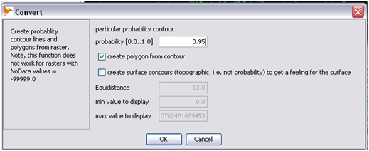Figure 7: Calculating Probability Contour

This should produce an image with 95% probability contour.

h_(ref, Gaussian)

Step 1: Open Kernel Density

Step 2: Fill in requried parameters as shown. Value 3828.754 is the h_ref value from h_(ad-hoc, Gaussian)

Figure 10: Calculating h_(ref,Gaussian)

Step 3: Create probability contour

h_(ref, Biweight)

This can be done by following the same step as h_(ref,Gaussian)

Except the requried parameters will have to be filled differently as shown below

Figure 11: Calculating h_(ref,Biweight)

h_(LSCV, Biweight)

Steps are the same as before, but with different parameters

Figure 11: Calculating h_(LSCV,Biweight)

Line-Buffer

Step 1: In 'MOVEAN' select 'Line Buffer HR'

Step 2: Fill out required parameters as follows

Figure 12: Calculating Line Buffer Home Range

Step 3: Create Probability Contour

LoCoH

NOTE: Apporpriate 'Parameter Value' is found by trial and error. Layer with the apporpriate value will produce an image that is similar to the images produced by other methods

LoCoH - a

Step 1: In 'MOVEAN' select 'LoCoH Home Ranges'

Figure 13: Calculating LoCoH-a Home Range

LoCoH - k

Repeat steps above. Select LoCoH - k

Figure 13: Calculating LoCoH-a Home Range

LoCoH - r

Repeat steps above. Select LoCoH - r

Figure 13: Calculating LoCoH-a Home Range

Line-Based Kernel Density

Step 1: Select 'Display Day Travel Ranges' from 'MOVEAN'

Figure 14: Calculating Daily Travel Range

Copy down the 'daily traveldist median' from the output window.

Step 2: Select 'Line-based Kernel Density for Movement Points' in 'MOVEAN

Step 3: Fill in the requirements. Bandwidth would be the daily traveldist median calculated from above

Figure 15: Calculating Line-based Kernel Density

Brownian Bridge

Step 1: In 'MOVEAN' select 'Display Liker Function for BB'

Step 2: Fill out requirments as shown below

Figure 16: Liker Function

Step 3: Copy down the minima Sigma. This will be the vaule of sigma 1 in Brownian Bridge

Step 4: In 'MOVEAN' select 'Brownian Bridge Home Ranges - Vector Segment Version'

Step 5: Fill our the required parameters as below

Figure 17: Calculating Brownian Bridge

Reflection

In this section, each method will be evaluated based on the amount of time for it to complete its calculation and the accuracy of the final image. Problems encountered with some methods will also be discussed.

MCP

Overall the program for MCP runs the fastest of all the calculation methods. However, the results produced by this method are not very accurate based on the fact that areas, such as mountain peaks and lakes that should not be covered by home range due to the fact that grizzlies would be very unlikely to appear in these conditions, were covered by this method